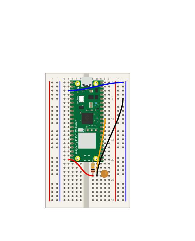
Measuring RC Filter Cutoff Frequency
Take the RC low-pass filter and pin down its cutoff frequency, the speed where the output amplitude falls to about 70.7% of the input. Predict fc = 1/(2πRC) for a 10 kΩ and 0.1 µF filter (about 160 Hz), then drive it at different speeds and watch the output swing shrink to confirm the trend and the −3 dB idea.
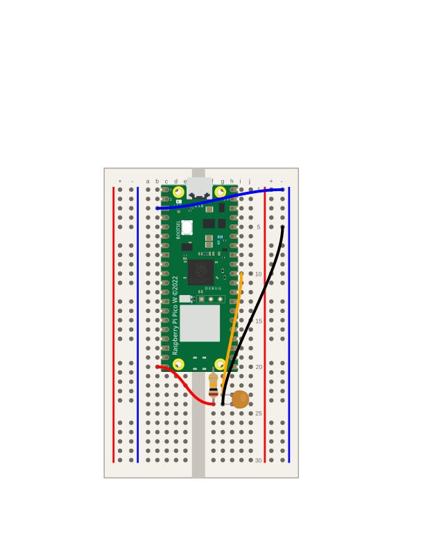
Build an RC Low-Pass Filter
Turn an RC circuit into a low-pass filter on the Pico W: drive it with a square wave from a GPIO, read the output with the ADC, and plot the commanded input beside the measured output. See intuitively why slow changes pass through while fast ones get smoothed away.
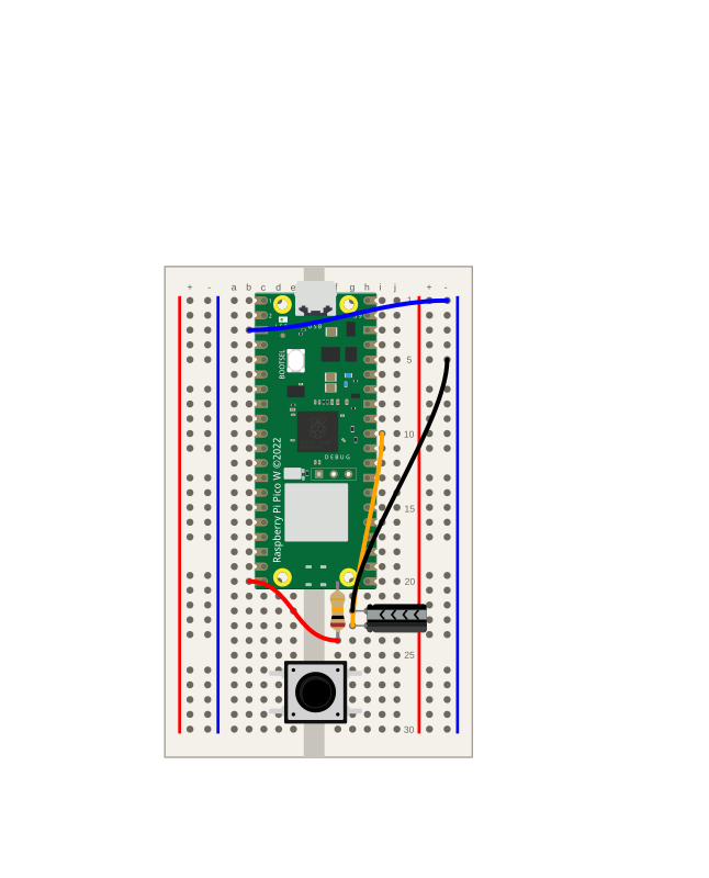
How Resistance and Capacitance Affect Charging Time
Keep the Pico W RC circuit and swap in different resistors and capacitors to see how each changes the charging time. Predict faster or slower with τ = R × C, measure the crossing at 2.09 V, and build a table confirming that more R or more C means a longer charge.
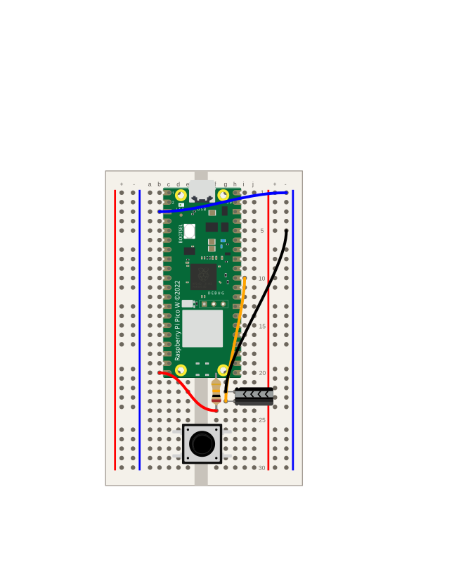
Measuring the RC Time Constant
Reuse the Pico W resistor–capacitor circuit to measure the time constant τ = RC: find when the capacitor reaches ~63.2% of the supply, then compare your measured τ against the calculated one.
Measuring Capacitor Charge and Discharge
Build a resistor–capacitor circuit on the Pico W, measure the capacitor's voltage with the ADC, and plot the charging and discharging curves over time.
pr-40
test

Using the Plotter
How to use the Plotter to view data in a line graph as it is printed from a device
Blinking the builtin LED using Micropython
how to make the built in led blink
Build an RC Low-Pass Filter
Build an RC Low-Pass Filter
What You'll Learn
- Turn an RC circuit into a low-pass filter.
- Drive it with a square wave from a Pico GPIO and watch the output with the ADC.
- See, intuitively, why slow (low-frequency) changes pass and fast ones are smoothed out.
What You'll Need
- Raspberry Pi Pico W on a half breadboard
- One 10 kΩ resistor
- One 0.1 µF ceramic capacitor — non-polarised, so no polarity to worry about
- A few jumper wires
- Comfortable measuring an RC circuit (the Measuring the RC Time Constant lesson) and reading a plot in the editor (the Using the Plotter lesson)
Background
Here's a question to sit with before you build anything. You're going to feed this circuit a square wave, a signal that jumps sharply between low (0 V) and high (3.3 V) over and over. When those jumps come slowly, only once every second or two, what do you think the output does? Now imagine the input flipping high and low hundreds of times a second. Does the output still follow every jump, or does something get lost?
A capacitor stores charge and can't change its voltage instantly, it always has to fill or empty through the resistor first. You saw that lag when you measured the charge and discharge curves. This lesson puts that same lag to work. A low-pass filter is a circuit that lets slow (low-frequency) changes through but smooths away fast (high-frequency) ones. Make your prediction for the slow case and the fast case now, then build the circuit and watch both play out on the plotter.
Build the Circuit
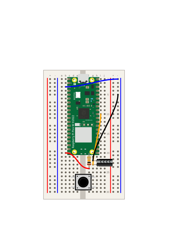
The filter is just a resistor in series feeding into a capacitor to ground. The Pico drives one end of the resistor with the square wave, the other end of the resistor joins the top of the capacitor to make the output node, and the ADC reads that node. The resistor and capacitor together decide how quickly the output node can follow the input.
- Place the 10 kΩ resistor so one leg is in hole
f24and the other inf23. - Connect the Pico's
GP15to the resistor leg in row 24. This end drives the filter with the square wave. - Place the 0.1 µF ceramic capacitor with one leg in row 23 (the same net as the resistor's other leg) and its other leg in row 22. The shared point in row 23 is the output node.
- Connect the Pico's
GP26to the output node in row 23.GP26is analog inputADC0. - Connect the capacitor's row-22 leg to the negative power rail.
- Connect a Pico GND pin to that same negative rail.
Note: A ceramic capacitor is non-polarised, it has no positive or negative leg, so it goes in either way round. That's a change from the electrolytic capacitor in the earlier lessons, where you had to watch the stripe and get the polarity right.
The output node sits between the resistor and the capacitor, driven from 3.3 V through the resistor, so its voltage always stays between 0 V and 3.3 V. That keeps it inside the safe range for the ADC pin, which must never see more than 3.3 V.
Write the Code
This program makes its own square wave on GP15: it flips that pin high and low in the loop, so the code always knows the input level it just commanded. Each pass it also reads the filter's output on GP26 and prints two numbers, the commanded input and the measured output, so the plotter draws them as two lines on one time axis. Type it into the editor and run it.
Python
from machine import Pin, ADC
import time

drive = Pin(15, Pin.OUT)   # GP15 drives the filter input through the 10 kOhm resistor
adc = ADC(26)              # GP26 / ADC0 reads the filter output (the RC node)

SAMPLE_STEP = 0.02          # seconds between readings (~50 samples per second)

# Set the square-wave speed by flipping the input every N samples. One half-cycle lasts
# N * SAMPLE_STEP seconds, so the drive frequency is about 1 / (2 * N * SAMPLE_STEP) Hz.
# N = 25 -> ~1 Hz,  N = 5 -> ~5 Hz,  N = 2 -> ~12.5 Hz.
SAMPLES_PER_HALF_CYCLE = 25

# Faithful waveforms only work at low frequencies (about 0.5 Hz up to a few tens of Hz),
# where each cycle gets several samples. Near and above the filter's cutoff the output
# stops tracing a clean wave and instead just looks smaller than the input, that shrinking
# is the point, and the next lesson digs into the cutoff frequency.

level = 1          # start driving the input high
count = 0          # samples counted in the current half-cycle

while True:
    drive.value(level)                          # command the input high or low
    v_in = level * 3.3                          # commanded input, in volts (0 or 3.3)
    v_out = adc.read_u16() * 3.3 / 65535         # measured output, in volts
    print("{:.3f},{:.3f}".format(v_in, v_out))  # CSV: input series, output series
    time.sleep(SAMPLE_STEP)                      # ~50 samples per second

    count = count + 1
    if count >= SAMPLES_PER_HALF_CYCLE:          # time to flip the square wave
        level = 0 if level else 1
        count = 0
Each line prints two numbers: the input voltage the code just drove, then the output voltage it measured. The plotter draws both as separate lines sharing one time axis, so you can watch the output next to the input that caused it. New to the plotter? See Using the Plotter.
How It Works
Think back to the charge and discharge curves. When the input jumped high, the capacitor didn't snap to 3.3 V, it climbed toward it, filling through the resistor. When the input dropped low, it eased back down. The capacitor always needs a little time to follow a change, because charge can only flow in or out through the resistor so fast.
That lag is the whole trick of a filter. When the input changes slowly, the capacitor has plenty of time to charge up and drain down between flips, so the output rides right along with the input, just with the sharp corners rounded off. But when the input changes quickly, the flips come faster than the capacitor can respond. Before it has finished charging toward high, the input has already dropped low again, and before it has drained, the input is back up. The output never reaches the top or bottom, it just wobbles gently around the middle. The fast wiggles get smoothed away while the slow trend still gets through, and that is exactly what "low-pass" means: low frequencies pass, high frequencies don't.
There's a particular changeover speed, called the cutoff frequency, where the output goes from mostly following the input to mostly getting smoothed out. The size of the resistor and the capacitor set where that changeover happens, just like they set the timescale of the charge curve. You don't need the exact number to see the effect here, the next lesson, RC Filter Cutoff Frequency, gives it a formula and shows you how to measure it.
SAMPLES_PER_HALF_CYCLE in the code is your speed dial. It decides how many samples the input holds high or low before flipping, so a smaller number means faster flips, a higher input frequency. Lowering it walks the input from slow to fast and lets you watch the output go from faithfully tracing the wave to barely twitching.
Try It
Run the program and watch the two lines on the plotter: the commanded input and the measured output, sharing one time axis.
- Start slow. With
SAMPLES_PER_HALF_CYCLE = 25(about 1 Hz) the output line tracks the input closely, a square wave with softened, rounded corners. The capacitor has time to charge nearly all the way to 3.3 V and drain nearly to 0 V on every flip, so the output swings almost as far as the input. - Speed it up. Lower
SAMPLES_PER_HALF_CYCLEto 5 (about 5 Hz), then to 2 (about 12 Hz), rerunning each time. Watch the output stop reaching the top and bottom, its swing shrinks and its corners round off more, until it's a small wobble near the middle while the input still jumps the full 0-to-3.3 V. - Record what you see at several settings: note the
SAMPLES_PER_HALF_CYCLEvalue and roughly how tall the output swing is compared to the input.
Note: Faithful side-by-side waveforms only work at low frequencies, where each cycle gets several samples. As you approach and pass the changeover speed, the plot stops being a clean traced wave and becomes an amplitude comparison, you're really just watching how much smaller the output swing is than the input. That shrinking is the point, and the next lesson leans into it.
Challenge
Predict before you measure. Somewhere between slow and fast there's a SAMPLES_PER_HALF_CYCLE value where the output clearly stops keeping up, its swing noticeably smaller than the input's. Write down your guess for that value first. Then test it: start high (slow) and step SAMPLES_PER_HALF_CYCLE down, rerunning each time, until the output visibly gives up on following the input. How close was your prediction?
Review
- When the input switches slowly, why does the output manage to follow it?
- When the input switches quickly, why can't the output keep up?
- Which passes through this filter more easily, low frequencies or high frequencies, and why?
- Lowering
SAMPLES_PER_HALF_CYCLEraises the input frequency. What did that do to the size of the output's swing?