Measuring RC Filter Cutoff Frequency
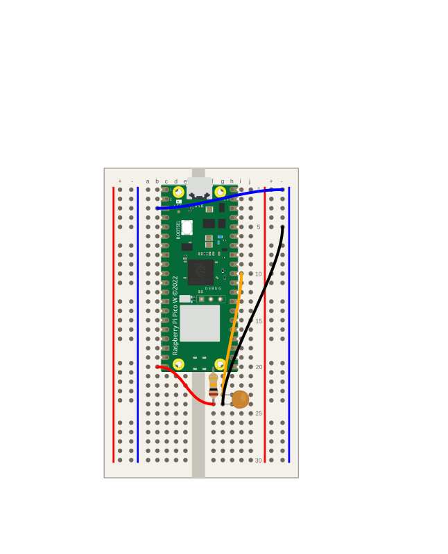
Take the RC low-pass filter and pin down its cutoff frequency, the speed where the output amplitude falls to about 70.7% of the input. Predict fc = 1/(2πRC) for a 10 kΩ and 0.1 µF filter (about 160 Hz), then drive it at different speeds and watch the output swing shrink to confirm the trend and the −3 dB idea.
Build an RC Low-Pass Filter
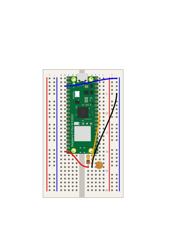
Turn an RC circuit into a low-pass filter on the Pico W: drive it with a square wave from a GPIO, read the output with the ADC, and plot the commanded input beside the measured output. See intuitively why slow changes pass through while fast ones get smoothed away.
How Resistance and Capacitance Affect Charging Time
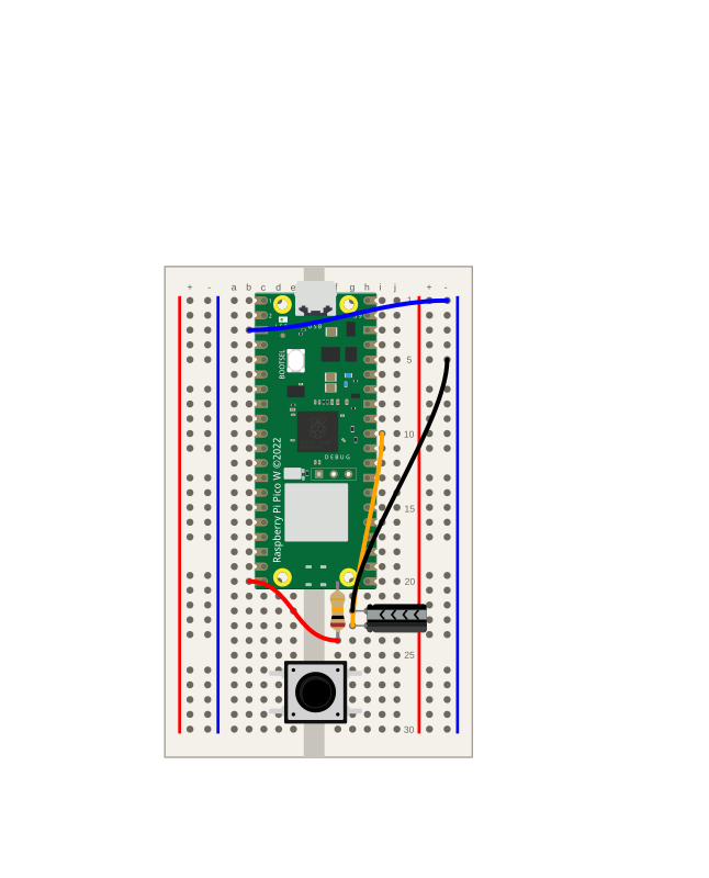
Keep the Pico W RC circuit and swap in different resistors and capacitors to see how each changes the charging time. Predict faster or slower with τ = R × C, measure the crossing at 2.09 V, and build a table confirming that more R or more C means a longer charge.
Measuring the RC Time Constant
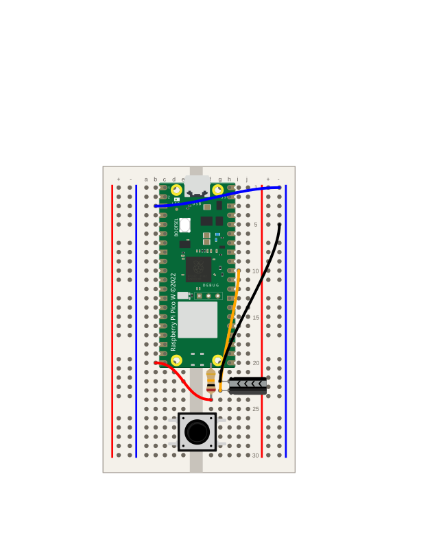
Reuse the Pico W resistor–capacitor circuit to measure the time constant τ = RC: find when the capacitor reaches ~63.2% of the supply, then compare your measured τ against the calculated one.
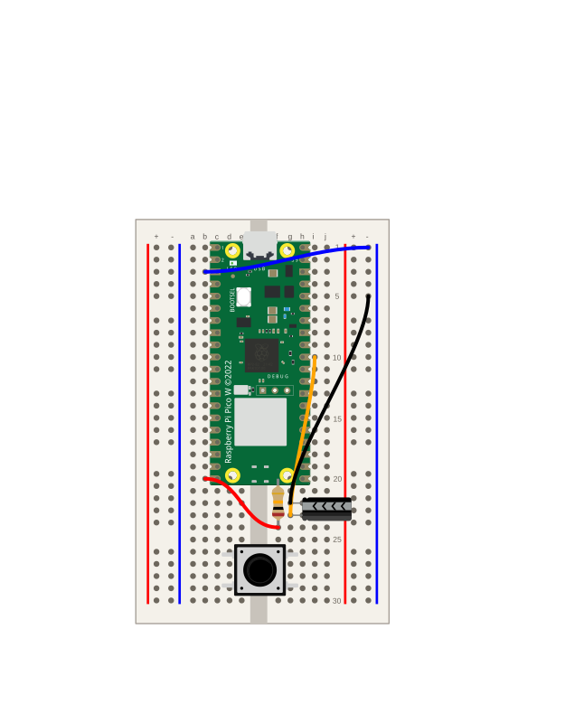
Measuring Capacitor Charge and Discharge
Build a resistor–capacitor circuit on the Pico W, measure the capacitor's voltage with the ADC, and plot the charging and discharging curves over time.
pr-40
test

Using the Plotter
How to use the Plotter to view data in a line graph as it is printed from a device
Blinking the builtin LED using Micropython
how to make the built in led blink
How Resistance and Capacitance Affect Charging Time
How Resistance and Capacitance Affect Charging Time
What You'll Learn
- How changing R and C changes the RC time constant, measured directly.
- Build a data table: R, C, calculated τ, predicted behaviour, measured τ, observations.
- The relationships: more R or more C → longer charge/discharge; less → shorter.
What You'll Need
- Pico W on a half breadboard, jumper wires
- A few resistor values (e.g. 1 kΩ, 10 kΩ, 22 kΩ) and a few electrolytic capacitor values (e.g. 10 µF, 100 µF, 1000 µF); the 10 kΩ + 100 µF pair from the earlier labs is the baseline
- Finished Measuring the RC Time Constant, recommended
Background
In Measuring the RC Time Constant you gave the charging curve a name: the time constant τ = R × C, the number of seconds it takes the capacitor to reach about 63.2% of the supply. That lesson used one resistor and one capacitor. Here you keep the same circuit but swap in different resistors and capacitors, run after run, to see how each choice changes the timescale.
Before you touch a part, make a prediction. τ = R × C, so the time constant scales with both R and C: make either one bigger and the capacitor takes longer to charge; make either one smaller and it charges faster. That gives four relationships to confirm by measurement:
- more resistance → longer charge time (bigger R stretches τ out)
- less resistance → shorter charge time (smaller R shrinks τ)
- more capacitance → longer charge time (bigger C stretches τ out)
- less capacitance → shorter charge time (smaller C shrinks τ)
Take the baseline of 10 kΩ and 100 µF, which gives τ = 1 second. Now predict, for each combination you plan to try, whether it will charge faster or slower than that baseline, and by roughly how much. For example, swapping the 10 kΩ for a 22 kΩ resistor should make the charge take a bit more than twice as long, because 22 kΩ is a bit more than double 10 kΩ. Write your faster/slower guesses down now — you'll fill in the measured times next to them and see whether the relationships hold.
Build the Circuit
This is the same circuit you built in Measuring Capacitor Charge and Discharge and Measuring the RC Time Constant: a resistor from a driving pin to the capacitor, with an analog pin reading the capacitor's voltage. Nothing about the wiring changes between runs — only the values of the resistor and capacitor you plug in. If the circuit is still on your breadboard, you can reuse it as-is; otherwise wire it up again:
- Place the resistor so one leg is in hole
f24and the other inf23. - Connect the Pico's
GP15to the resistor leg in row 24. This end drives the circuit. - Place the capacitor with its positive leg in row 23 (the same net as the resistor's other leg) and its negative leg in row 22. Row 23 is the node you measure.
- Connect the Pico's
GP26to the capacitor's positive leg.GP26is analog inputADC0. - Connect the capacitor's negative leg to the negative power rail.
- Connect a Pico GND pin to that same negative rail.
The diagram (in the lesson's repository) shows the baseline parts (10 kΩ and 100 µF), but the layout is identical for every combination in this lesson. To try a new combination, power down, pull the resistor or capacitor, drop in the new value in the same holes, and run again. Keep the polarity and holes exactly as shown; only the part values differ.
Warning: The electrolytic capacitor is polarised. Its negative leg (usually the shorter one, marked with a stripe) goes to ground. Putting it in backwards can damage it — double-check the orientation every time you swap a capacitor.
The measured node only ever charges from 3.3 V through the resistor, so its voltage stays between 0 V and 3.3 V — safely inside the ADC's limit, which must never see more than 3.3 V.
Write the Code
This is the same measurement you used in Measuring the RC Time Constant, but now you run it once per R/C combination. It empties the capacitor, drives GP15 high to charge it through the resistor, and prints the voltage many times a second for the plotter. It also watches for the moment the voltage first crosses 63.2% of 3.3 V (about 2.09 V) — that crossing time is your measured τ for this combination.
Because R and C change from run to run, you set them at the top of the program in R_OHMS and C_FARADS. The code then prints both the calculated τ = R × C for the parts you entered and the measured τ it timed. Update those two values before each run so every row of your table comes from one run with the parts you actually installed.
Python
from machine import Pin, ADC
import time

# --- Set these to match the parts you installed for THIS run -------------------
# Update R_OHMS and C_FARADS every time you swap a part, so the calculated tau the
# code prints matches the resistor and capacitor actually on the breadboard. Each
# row of your table comes from one run with one combination.
R_OHMS = 10_000        # resistor value in ohms   (e.g. 10_000 for 10 kOhm)
C_FARADS = 100e-6      # capacitor value in farads (e.g. 100e-6 for 100 uF)
# -------------------------------------------------------------------------------

drive = Pin(15, Pin.OUT)   # GP15 drives the RC network through the resistor
adc = ADC(26)              # GP26 / ADC0 reads the voltage on the RC node

SAMPLE_STEP = 0.02          # seconds between readings (~50 samples per second)

SUPPLY = 3.3                # volts driven onto the network
TARGET_FRACTION = 0.632     # one time constant reaches ~63.2% of the final voltage
TARGET_VOLTS = SUPPLY * TARGET_FRACTION   # ~2.09 V at a 3.3 V supply

CALCULATED_TAU = R_OHMS * C_FARADS        # R * C, in seconds

# Watch for about 5 time constants so the curve has room to flatten out. Give slow
# combinations enough time, but always watch at least a couple of seconds.
CHARGE_TIME = max(2, 5 * CALCULATED_TAU)  # seconds to watch the capacitor charge


def read_volts():
    # read_u16() gives 0-65535; scale it to the 0-3.3 V the ADC measures
    return adc.read_u16() * SUPPLY / 65535


# Start from empty: drive GP15 low so the capacitor discharges fully before we time it.
drive.value(0)
time.sleep(CHARGE_TIME)

# Charge: drive GP15 high so the capacitor fills up through the resistor.
drive.value(1)
start = time.ticks_ms()
measured_tau = None   # filled in the first time we cross TARGET_VOLTS

while time.ticks_diff(time.ticks_ms(), start) < CHARGE_TIME * 1000:
    t_ms = time.ticks_diff(time.ticks_ms(), start)   # milliseconds since charging began
    volts = read_volts()
    print("{},{:.3f}".format(t_ms, volts))            # CSV: t_ms,volts

    # The first sample at or above 2.09 V marks one time constant.
    if measured_tau is None and volts >= TARGET_VOLTS:
        measured_tau = t_ms / 1000   # convert milliseconds to seconds

    time.sleep(SAMPLE_STEP)

# Print both taus for this combination: what R * C predicts, and what we timed.
if measured_tau is not None:
    print("# calculated tau = {:.2f} s, measured tau = {:.2f} s".format(
        CALCULATED_TAU, measured_tau))
else:
    print("# never reached {:.2f} V - charge longer or check the wiring".format(
        TARGET_VOLTS))
How It Works
The program is the τ measurement from Measuring the RC Time Constant, wrapped so you can run it once per combination. It empties the capacitor, drives GP15 high to charge it through the resistor, prints the voltage many times a second for the plotter, and records the instant the voltage first crosses 2.09 V (63.2% of 3.3 V) as the measured τ. The two values at the top, R_OHMS and C_FARADS, tell the code which parts are on the board so it can print the calculated τ = R × C alongside the measured one.
That side-by-side is the whole point. For each combination the code hands you two numbers: what R × C predicts, and what the circuit actually did. Because τ = R × C, the calculated value moves in lockstep with the parts:
- Double the resistance and τ doubles. 22 kΩ with 100 µF gives τ ≈ 2.2 s, a bit over twice the 1 s baseline — so the curve should take a bit over twice as long to reach 2.09 V.
- Change the capacitance the same way and τ tracks it too, because C multiplies in exactly like R does. Ten times the capacitance means ten times the time constant.
So each row of the table below is a small test of τ = R × C: the measured crossing time should land close to the calculated R × C for the parts you installed. When they agree across several very different combinations, you've confirmed the four relationships from the Background — more R or more C stretches the curve out, less R or less C pulls it in — and seen that τ scales linearly with both.
Try It
Work through a set of combinations, one run each. For every row, calculate τ = R × C first and predict whether it charges faster or slower than the 1 s baseline. Then set R_OHMS and C_FARADS to match the parts, run the program, read the measured τ off the summary line (or the plot), and note what you saw.
Plain Text
R        | C       | Calculated tau = R x C | Predicted vs baseline | Measured tau | Observations
-------- | ------- | ---------------------- | --------------------- | ------------ | ------------------------------------------------
10 kOhm  | 100 uF  | 1.0 s                  | baseline              | ___ s        | starting point; curve reaches 2.09 V at ~1 s
22 kOhm  | 100 uF  | 2.2 s                  | slower (more R)       | ___ s        | bigger R -> longer; ~2.2x the baseline
1 kOhm   | 100 uF  | 0.1 s                  | faster (less R)       | ___ s        | smaller R -> shorter; crosses quickly, watch closely
10 kOhm  | 10 uF   | 0.1 s                  | faster (less C)       | ___ s        | smaller C -> shorter; same fast crossing as 1k + 100uF
10 kOhm  | 1000 uF | 10 s                   | slower (more C)       | ___ s        | bigger C -> longer; be patient, this one takes a while
1 MOhm   | 1000 uF | 1000 s (~17 min)       | far slower            | predict only | reasoning row: tau is huge, so charging crawls
Fill the Measured τ column from your runs and compare it to the calculated column beside it. They should track each other closely; small gaps are normal, since real parts vary from their labels and the ~50 Hz sampling only catches the crossing to within one reading. The faster combinations (τ = 0.1 s) cross 2.09 V in a handful of samples, so read those from the printed summary rather than trying to eyeball the plot.
The last row is deliberately impractical. With 1 MΩ and 1000 µF, τ = 1,000,000 Ω × 0.001 F = 1000 seconds — about 17 minutes to reach 2.09 V, and roughly an hour and a half to look fully charged. You don't build or time that one; you reason about it. It's the same rule taken to an extreme: pile on resistance and capacitance and the charge time grows without limit. That's why practical RC timing circuits stay in the range you can actually measure.
Look across your filled-in rows and confirm all four relationships hold: more R made it slower, less R faster, more C slower, less C faster — and the size of the change matched how much you scaled R or C.
Challenge
Turn the rule around: instead of picking parts and finding τ, pick a target τ and choose parts to hit it. Say you want a time constant of half a second (τ = 0.5 s). Which resistor and capacitor from your kit multiply to R × C = 0.5 s? There's more than one answer — for instance 5 kΩ × 100 µF, or 10 kΩ × 50 µF. Pick a pair, predict where the curve should cross 2.09 V (right around 0.5 s), then set R_OHMS and C_FARADS, run it, and check your measured τ against the 0.5 s target. Try a second target, like τ = 3 s, and see how close you can get with the parts you have.
Review
- τ = R × C. If you double the resistance and leave the capacitor alone, what happens to the time constant?
- If you halve the capacitance and leave the resistor alone, what happens to the time constant?
- State the four relationships in your own words: what does more R, less R, more C, and less C each do to the charge time?
- Why is the 1 MΩ + 1000 µF combination a prediction-only exercise rather than something you measure?